AWS from Zero to Production — Phase 9, Part 5 of 11 · See the full series roadmap
Athena is brilliant for exploring the lake. But then the business wants dashboards — dozens of them, refreshed constantly, used by hundreds of people, with complex joins across many tables, and answers in under a second.
Running all of that on Athena, scanning S3 on every click, gets slow and expensive. That’s when you reach for a data warehouse.
Amazon Redshift is AWS’s cloud data warehouse: columnar storage, massively parallel processing, a SQL interface your BI tools already speak — and deep integration with your S3 lake.
What you’ll walk away with
- 🏛️ Data warehouse concepts
- ☁️ Redshift Serverless vs. provisioned clusters
- 🧮 Distribution styles, sort keys, and compression encoding
- 📥 COPY and UNLOAD
- 🔭 Redshift Spectrum
- 🚦 Workload management
- 🪞 Materialized views and data sharing
- 🔐 Security and performance tuning
Data warehouse concepts
A warehouse stores modeled, cleaned data for analytics. Common modeling patterns:
- Fact tables — events and measurements: orders, payments, page views. Long and narrow.
- Dimension tables — context: customers, products, dates, regions. Shorter and wider.
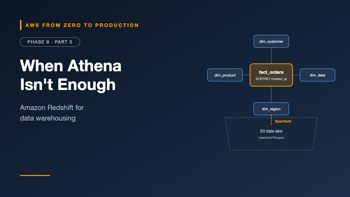
- Star schema — a fact table surrounded by dimensions it joins to.
             dim_customer
                  |
dim_product -- fact_orders -- dim_date
                  |
             dim_region
Redshift stores data by column, compresses it heavily, and splits queries across many compute slices that work in parallel — MPP (massively parallel processing).
Redshift Serverless vs. provisioned clusters
Redshift Serverless
- No clusters to size or manage. Capacity is measured in Redshift Processing Units (RPUs) and scales automatically.
- A namespace holds your databases, users, and data; a workgroup holds compute settings — base capacity, network, and limits.
- Pay for RPU-hours used while queries run, plus storage. Set a maximum RPU limit to cap spend.
- Best for: new workloads, variable or unpredictable usage, dev and test.
Provisioned clusters
- You choose a node type — RA3 for new clusters — and node count.
- RA3 separates compute from storage with Redshift Managed Storage, so you scale them independently.
- Pay per node-hour, with Reserved Instances for steady workloads.
- Best for: steady, predictable, high-utilization workloads where you want fine control.
Default choice: Start with Redshift Serverless. Consider provisioned clusters once usage is steady and well understood.
Table design
Three choices drive Redshift performance: distribution, sort keys, and compression.
Distribution styles
Distribution decides which slice stores each row. Joins are fastest when matching rows live on the same slice.
- AUTO (default) — Redshift chooses and adjusts. A good default.
- KEY — rows with the same value in the distribution key go to the same slice. Use for large tables you join on that key, like
customer_idon bothfact_ordersanddim_customer. - ALL — a full copy on every node. Use for small, frequently joined dimension tables.
- EVEN — round-robin. Use when there’s no clear join key.
Watch out: A KEY column with skewed values — like a few customers owning most orders — puts most data on a few slices, and they become the bottleneck.
Sort keys
A sort key stores rows in order. Redshift keeps min and max values per block, and skips blocks that can’t match — like partition pruning, inside the table.
- Pick columns used in range filters — usually dates.
- Compound sort keys work best when queries filter on the leading column.
- AUTO lets Redshift choose based on query patterns.
Compression encoding
Each column is compressed with an encoding — like AZ64 for numbers and dates, and ZSTD or LZO for text. With ENCODE AUTO (the default), Redshift chooses for you.
CREATE TABLE fact_orders (
  order_id     BIGINT,
  customer_id  BIGINT,
  item         VARCHAR(200),
  total        DECIMAL(12,2),
  created_at   TIMESTAMP
)
DISTSTYLE KEY
DISTKEY (customer_id)
SORTKEY (created_at);
COPY: loading data
COPY loads data from S3 in parallel across all slices. It’s far faster than INSERT statements:
COPY fact_orders
FROM 's3://acme-lake-curated/sales/orders/'
IAM_ROLE default
FORMAT AS PARQUET;
- Supports Parquet, ORC, Avro, JSON, and CSV.
- Split large input into many files — ideally a multiple of the number of slices — so every slice works.
- Uses an IAM role attached to the warehouse; no keys in SQL.
- Auto-copy can load new files automatically as they land in S3.
UNLOAD: exporting data
UNLOAD writes query results back to S3, in parallel:
UNLOAD ('SELECT order_date, COUNT(*) AS orders FROM fact_orders GROUP BY 1')
TO 's3://acme-lake-consumption/sales/daily_orders/'
IAM_ROLE default
FORMAT AS PARQUET
PARTITION BY (order_date);
Use it to share warehouse results with the lake, ML pipelines, or other teams.
Redshift Spectrum: query the lake from the warehouse
Spectrum lets Redshift query data in S3 directly, through the Glue Data Catalog:
CREATE EXTERNAL SCHEMA lake
FROM DATA CATALOG
DATABASE 'sales_curated'
IAM_ROLE default;

SELECT d.region, SUM(o.total)
FROM lake.orders o            -- in S3
JOIN dim_region d             -- in Redshift
  ON o.region_id = d.region_id
WHERE o.order_date >= '2026-10-01'
GROUP BY d.region;
The pattern this enables:
- Hot, frequently queried data lives in Redshift.
- Large, historical, or rarely queried data stays in S3.
- One SQL query joins both.
Workload management (WLM)
Not every query is equally important. Workload management decides how queries share resources:
- Automatic WLM (the default on provisioned clusters) manages memory and concurrency for you.
- Query priorities — so the CFO’s dashboard beats an analyst’s ad hoc exploration.
- Query monitoring rules — log, abort, or deprioritize queries that run too long or scan too much.
- Concurrency scaling — adds temporary capacity for bursts of concurrent queries.
- Short query acceleration — runs quick queries ahead of long ones.
Redshift Serverless handles scaling automatically, with usage limits and query limits to control cost and runaway queries.
Materialized views
A materialized view stores the precomputed result of a query:
CREATE MATERIALIZED VIEW mv_daily_revenue
AUTO REFRESH YES
AS
SELECT DATE_TRUNC('day', created_at) AS day, SUM(total) AS revenue
FROM fact_orders
GROUP BY 1;
- Dashboards query the small result instead of the huge table.
- Incremental refresh updates only what changed, where supported.
- Automatic query rewriting can use a materialized view even when a query targets the base table.
Data sharing
Data sharing gives other Redshift warehouses live, read-only access to your data — with no copying:
- Share across warehouses, accounts, and Regions.
- Producers and consumers use separate compute, so a heavy consumer can’t slow down the producer.
- Share specific schemas, tables, or views.
A common pattern: one ETL warehouse loads and models data; separate BI and data science warehouses consume it through data shares.
Redshift security
- Network: deploy in private subnets; turn off public accessibility.
- Encryption: at rest with KMS, and in transit with TLS — require SSL.
- Authentication: IAM, identity provider federation, or IAM Identity Center. Let Redshift manage the admin password in Secrets Manager.
- Authorization: role-based access control (RBAC), and column-level grants.
- Row-level security — policies that filter rows by user or role.
- Dynamic data masking — mask sensitive columns, like showing only the last four digits of a card number, based on role.
- Auditing: audit logs to CloudWatch or S3, plus CloudTrail for API calls.
Integration with S3 and Glue
Redshift fits the lakehouse:
- COPY from and UNLOAD to S3.
- Spectrum queries Glue catalog tables in S3.
- Reads and writes Iceberg tables in S3.
- Zero-ETL integrations replicate data from Aurora, RDS, and DynamoDB into Redshift continuously, without building a pipeline.
- Query editor v2 in the console, and the Data API for running SQL from Lambda, Step Functions, or scripts — without managing connections.
aws redshift-data execute-statement \
  --workgroup-name analytics \
  --database dev \
  --sql "SELECT COUNT(*) FROM fact_orders"
Performance tuning
- Let AUTO do its job for distribution, sort keys, and encoding — and check its recommendations with Advisor.
- Filter on sort key columns.
- Join on distribution keys, and use
DISTSTYLE ALLfor small dimensions. - Avoid
SELECT *— columnar storage rewards narrow selects. - Load with
COPY, never row-by-row inserts. - Use materialized views for repeated aggregations.
- Check
EXPLAINfor redistribution steps (DS_BCAST_INNER,DS_DIST_BOTH) that move data between nodes. - Vacuum and analyze are mostly automatic now, but check table health in system views like
SVV_TABLE_INFO.
Athena or Redshift?
- Athena: ad hoc exploration, infrequent queries, data that’s mostly in the lake, and no infrastructure at all.
- Redshift: many concurrent users, BI dashboards, complex joins, sub-second performance, and modeled warehouse data.
Most platforms use both — on the same S3 data and the same catalog.
Common mistakes
- Row-by-row
INSERTs instead ofCOPY. - Skewed distribution keys.
- No sort key on date-filtered fact tables.
- Publicly accessible warehouses.
- No usage limits on Serverless.
- Copying all data into Redshift when Spectrum would do for cold data.
- Dashboards querying huge base tables instead of materialized views.
Key takeaways
- Redshift is a columnar, MPP warehouse for fast, concurrent analytics.
- Start with Serverless; consider provisioned RA3 for steady workloads.
- Distribution, sort keys, and compression drive performance — AUTO is a strong default.
- COPY loads in parallel; UNLOAD exports; Spectrum queries the lake.
- Materialized views and data sharing serve many consumers efficiently.
- Lock it down: private networking, encryption, RBAC, row-level security, and masking.
Quick self-check
Test yourself before moving on:
- Which distribution style suits a small, frequently joined dimension table?
- Why is
COPYfaster thanINSERT? - How can Redshift query historical data that stays in S3?
- What feature masks a credit card column for most users but not for the fraud team?
Answers
DISTSTYLE ALL.- It loads in parallel across all slices, from many files at once.
- Redshift Spectrum, through the Glue Data Catalog.
- Dynamic data masking.
What’s next
In Part 6, we scale processing: Amazon EMR and Apache Spark — EMR on EC2, Serverless, and EKS, partitioning and shuffles, data skew, memory, Spot Instances, and troubleshooting.
Redshift, Snowflake, BigQuery, or something else — what’s your team’s warehouse? Tell me in the comments.